

by Neel Kaila, Director, Neel Pty Ltd, Nathaniel Brubaker, Engineering Student, Miami University and Robbert Veerman, Technical Consultant
At its simplest, a hydraulic system converts mechanical energy into fluid flow and pressure in order to complete a specified amount of work. In general, the less energy lost in this process, the more energy efficient the system will be. However, hydraulic systems often lose pressure along pipelines, which can have substantial implications for the energy efficiency and operating costs of the system as a whole. This article explores the concept of pressure recovery in hydraulic systems and presents a solution for energy recovery in pipelines with a siphon leg of more than 10 metres, through the use of a hydraulic turbine.
Understanding the hydraulic number line
A hydraulic number line is instrumental when exploring concepts of pressure loss and recovery in a system.
However, to understand the hydraulic number line, it is useful to first look at a mathematical number line, which depicts the possible values of all real numbers (Figure 1).
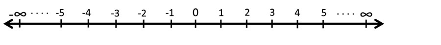
Figure 1.
The same basic idea can be applied to create a number line for hydrostatics, representing all possible pressure head values available to a hydraulic system (Figure 2).
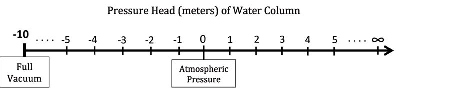
Figure 2.
However, unlike the mathematical number line, the hydraulic number line has a lower limit.
The hydraulic number line only includes negative values down to approximately -10. This means that any values below -10 do not exist in the hydraulic number line, because they are not possible in hydraulic systems.
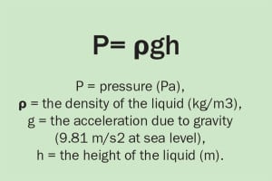
The values of the hydraulic number line refer to the pressure head, also called the static head, of a system. Pressure head is the internal energy of an incompressible liquid due to the pressure it exerts on its container, proportional to the height of an equivalent column of static liquid. Head is measured by length, typically metres. Although head refers to the height of a column of liquid, it has a direct relation to pressure:
The reason for the lower limit
The lower limit of the hydraulic number line was defined by Italian physicist Evangelista Torricelli, best known for his contributions to hydrodynamics and his invention of the barometer.
Torricelli’s experiment involves filling a tube with liquid mercury (ρ = 13.6 kg/m3) and plugging both ends. One end of the tube is then placed in a basin, already filled with water, and the submerged plug is removed. At this point, some of the liquid will flow out of the tube into the basin until a point of equilibrium is reached.
This occurs because atmospheric pressure pushes the column of liquid up the enclosed tube until it reaches an adequate height to balance the atmospheric pressure. The barometer acts as a balance between the weight of liquid and atmospheric pressure.
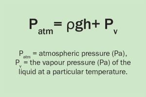
The equation to calculate the atmospheric pressure is:
During his work with barometers, Torricelli noticed that there was a limit to the height that a liquid could reach. When the bottom of the tube was unplugged, only part of the liquid would flow out and no matter how long the tube was the liquid would settle at the same height every time.
The only variation in these circumstances was the size of the void or vacuum space created at the top of the tube. If the experiment is altered and the barometer is filled with water, the same thing occurs.
This phenomenon can be explained by looking at the formula used to calculate atmospheric pressure (Equation 2). If density, temperature, vapour pressure and atmospheric pressure remain constant, then the height of liquid will never change. The maximum height that a column of water (ρ = 1000 kg/m3) can reach in an open system under normal atmospheric pressure is ten metres. This is shown when you rearrange the equation for atmospheric pressure:
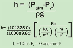
Note: For the purposes of calculation, frictionless pipework and a vapour pressure of zero is assumed.
The calculated value of ten metres corresponds to the lower limit of the hydraulic number line, -10.
This means the air pressure outside the column is sufficient to drive water to a height of ten metres up the column. The space in the column above the water exerts no influence since there is zero vapour pressure. If the relation between head and water height is once again established, at nine metres above the external water level the pressure head will be -9m, a height of four metres up will correspond to a -4m head, and so on.
Applying the hydraulic number line to a hydraulic system
To apply the hydraulic number line to a hydraulic system, such as a barometer, rotate the hydraulic number line (Figure 2) so that the lower limit of -10 points upwards and the upper limit (∞) points down. Then align the zero point of the number line with the hydraulic grade line (HGL) of the tank (Figure 3). With the correct units, the values represent the pressure head, or potential energy, at a particular height.
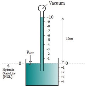
Figure 3.
As the barometer displays, the hydraulic value decreases from zero moving up the tube and increases infinitely moving deeper into the tank.
Calculating pump head
A. For a hydraulic system with a siphon leg <10 metres
The application of the hydraulic number line principle is extremely helpful when calculating hydrostatic head (potential energy change). In a hydraulic pump system, total pump head equates to the linear vertical measurement of the height a specific pump can deliver a liquid at the pump discharge. The pump head can be calculated by measuring the differential head across a pump:

Note: To simplify, the authors have assumed zero friction loss. The reader can add friction head to obtain total pump head.
In order to calculate the pump head of a simple system, three simple steps must be followed.
1. Set the hydraulic grade line or baseline at a head of zero.
2. Assign the corresponding positive or negative head values depending on whether the system proceeds down or up, using the hydraulic number line and the same technique as with the barometer. This process of adding or subtracting head is continued throughout the system until the pump nozzle is reached.
3. Take the final values at the suction and discharge of the pump and subtract the two to obtain the total pump head (once again friction losses are assumed to be zero).
To further demonstrate the calculation of pump head, a simple hydraulic pump system can be examined (Figure 4). The example system has two open tanks filled to the same height (elevation), each with a depth of two metres, is open to the atmosphere, and has one pump and an inverted U-shaped configuration that extends to a height of eight metres.
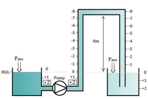
Figure 4.
First, HGL is set to a head of zero metres. The second step involves moving from the atmosphere to the pump, tracing the path that is taken and determining pressure head at each stage. On the left tank, head increases two metres down to the pump, giving the suction head a value of +2m. In the right tank, the liquid rises eight metres from the water level, resulting in a head of -8m at the top of the system.
The pressure head remains constant throughout the horizontal section (as there is no change in elevation), and then increases as we move towards pump discharge. Once the elevation decreases again, the amount of the liquid above increases and the pressure head will increase accordingly. While the column of water above continues to grow, the associated head increases from -8m to +2m as the liquid experiences the ten-metre elevation change. The final pressure head at the pump discharge is +2m.
The suction head and discharge head are now established as +2m. In the final step, the total pump head of the system can be calculated by the difference between the discharge head and suction head and adding the friction losses.
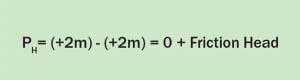
B. For a hydraulic system with a siphon leg >10 metres
Calculating the pump head of a taller system (i.e. >10m) results in a different answer.
However, the equation for calculating pump head itself does not change; it remains the differential of heads across the pump.
Consider a system, similar to the last, that has two open tanks with depths of two metres, except the system reaches a height of 18 metres instead of eight metres.
Follow the same steps as before to calculate the pump head of the system. Start with the system’s interaction with the atmosphere and set the elevation as a head of zero. Second, determine the pressure on either side of the pump. Note that the suction head has not changed from the previous configuration, remaining at +2m.
The calculation of the minimum required operating discharge head begins at the right tank. Using the hydraulic number line, the pressure head will increase negatively until a head of -10m is reached at a height of 10m. At this point the hydraulic number line ends because full vacuum is reached; there is nothing past -10m.
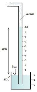
Figure 5.
Above the maximum height of the water column, the vacuum extends all the way to the top of the system (Figure 5). Head remains constant at -10m until the elevation starts to drop in the downward leg and the weight of water is able to increase the pressure once more. This is evident on the other side of the U-shaped configuration where the vacuum ceases, and the head increases. The conventional method of counting proceeds from there and the pump is reached with a discharge head of +7m.

Figure 6.
Looking at the entire system (Figure 6), we can see that the suction head is +2m and discharge head is +8m. The total pump head of this system can be calculated by the difference in the new suction and discharge heads.
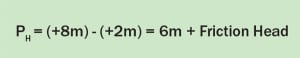
The total pump head of this system is calculated to be +6m. This means that in order for the system to operate, the pump must produce a head of six metres. This value is obviously different from the pump head achieved in the previous system with a siphon leg of less than ten metres (Figure 4).
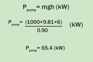
If the mass flow rate of the system in Figure 6 is 1,000 kg/sec and the pump has an efficiency of 90 per cent, then the pump power, Ppump, for this system can be calculated.
Pressure recovery in hydraulic systems
A. For a hydraulic system with siphon leg >10 metres
Now that we have examined the systems, the question remains of how this energy can be recovered.
Recovery can be achieved by introducing a hydraulic turbine. This will allow the system to capture work done by liquid falling onto the turbine. If the turbine is then connected to a generator or reconnected to the pump shaft, part of this energy can then be returned to the system.
In this next example, the turbine produces power at a +6m head differential (Figure 7).
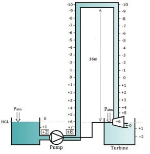
Figure 7.
At the HGL, there is a head of zero metres, but since the turbine is placed at that point, head increases to +6m. The head continues to decrease by conventional counting, only reaching a value of -10 m at the apex of the pipe length and ending with a pump discharge head of +8m.
The work done by the fluid on the turbine is then converted directly to usable energy to the pump. As a result, some of the energy that would otherwise be lost is restored to the system.
The pump’s head value remains the same, but the energy required to produce that head is partly recovered by the turbine (note that in this example the pump and turbine are on a common shaft). Simply introducing a pressure differential by means of a turbine eliminates the vacuum region and allows you to take advantage of the work produced by falling water. A somewhat similar process occurs in certain turbocharger pressure recovery units in internal combustion engines.
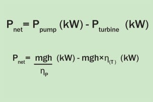
To quantify the power saved by a pressure recovery turbine, the power generated by the turbine should be subtracted from the power consumed by the pump. In this case, both pump and turbine have an assumed efficiency of 90 per cent.
B. A real life application of a pressure recovery turbine
To look at how a pressure recovery turbine can be used in a real life application, we will use the example of a long distance pipeline (e.g. water supply lines to water treatment plants, mines, etc.). Commonly, such pipelines stretch many kilometres, over which they may encounter elevation changes greater than ten metres.
Consider the long distance pipeline in Figure 8, through which water is pumped from a reservoir to a local town ten kilometres away.
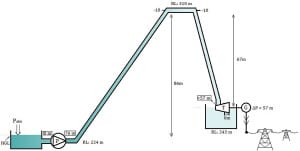
Figure 8.
The pump sits at an elevation of 224m, and along the transit the pipeline rises 76m to an elevation of 310m and finally drops 67m into a tank at 243m.
The turbine is placed at the grade line of the tank. The system has a steady flow of 1,000 kg/sec along (assumed) frictionless pipes.
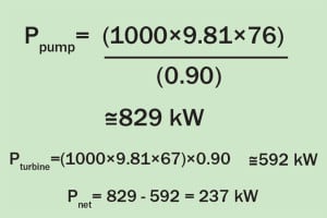
When this system is analysed using the number line principle the pump head is found to be 76m. For the sake of simplicity, the inlet for the pump is placed at the water’s surface so the suction head is considered zero. With 90 per cent efficiency, the power consumed by the pump is 829 kW. The head loss at the turbine is 67m. At 1,000 kg/sec, that equates to 592 kW of power generated.
This energy can then be fed into the local power grid for use by the community. Essentially, the turbine is recovering energy that would otherwise be lost. The turbine reduces the net energy loss of pumping water across long distances. Here there is a net power consumption of only 237 kW (829 – 592 kW), representing a substantial benefit to the operator.
Overall, the introduction of a turbine into appropriate hydraulic systems can result in substantial energy recovery and associated reductions in operating costs. The methods outlined in this article can be applied to other appropriate hydraulic systems to calculate the benefits that could be achieved by incorporating a turbine.


